BJT Amplifiers – Small Signal Analysis
$5.00
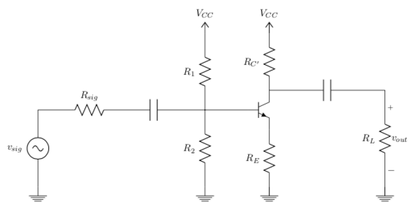
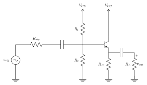
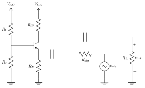
This document contains methods and proofs for determining multiple figures of merit to many configurations of Bipolar Junction Transistor amplifiers. These proofs are usually found in a course on Electronics. BJT amplifier configurations covered are the common emitter (with and without the emitter resistance), the common base (with and without the base resistance), and the common collector.
Description
Excerpt from the Common Emitter section of document (depicted in main image of this resource):
The first figure of merit we are asked to determine is \(R_{in}\).
We know from Figure 5 that \(R_{in}\) represents the entire amplifier to the right of \(R_{sig}\). We also know that \(R_{in} = \frac{v_{in}}{i_{in}}\). We can determine \(v_{in}\) and \(i_{in}\) from the circuit in Figure 10.
Writing a nodal equation for \(i_{in}\) yields:
\begin{align}
i_{in} &= i_{B} + i_{b} \nonumber \\
\textit{where } i_{B} &= \frac{v_{in}}{R_{B}} \nonumber \\
i_{in} &= \frac{v_{in}}{R_{B}} + i_{b}\ \ \ \ \ (2)
\end{align}
Writing a mesh equation for \(v_{in}\) yields:
\begin{equation}
v_{in} = i_{b}r_{\pi} + i_{e}R_{E}\ \ \ \ \ (3)
\end{equation}
Let’s continue to develop \(v_{in}\) by obtaining it in terms of \(i_{b}\) since Equation (2) is in terms of \(i_{b}\). We can accomplish this by writing a nodal equation for \(i_{e}\), where:
\begin{align}
i_{e} &= i_{b} + \beta{i_{b}} \nonumber \\
&= (\beta+1)i_{b}\ \ \ \ \ (4)
\end{align}
Subbing \(i_{e}\) in Equation (4) for \(i_{e}\) in Equation (3) yields:
\begin{align}
v_{in} &= i_{b}r_{\pi} + i_{b}(\beta+1)R_{E} \nonumber \\
&= [r_{\pi} + (\beta+1)R_{E}]i_{b}\ \ \ \ \ (5)
\end{align}
Solving for \(i_{b}\) in Equation (5) produces:
\begin{equation}
i_{b} = \frac{v_{in}}{r_{\pi} + (\beta+1)R_{E}}\ \ \ \ \ (6)
\end{equation}
Substituting Equation (6) into Equation (2) for \(i_{b}\) yields:
\begin{align}
i_{in} &= \frac{v_{in}}{R_{B}} + \frac{v_{in}}{r_{\pi} + (\beta+1)R_{E}} \nonumber \\
&= \left[\frac{1}{R_{B}} + \frac{1}{r_{\pi} + (\beta+1)R_{E}}\right]v_{in}\ \ \ \ \ (7)
\end{align}
Solving for \(\frac{i_{in}}{v_{in}}\) in Equation (7) yields:
\begin{equation}
\frac{i_{in}}{v_{in}} = \frac{1}{R_{in}} = \frac{1}{R_{B}} + \frac{1}{r_{\pi} + (\beta+1)R_{E}}\ \ \ \ \ (8)
\end{equation}
From circuit theory, we know that:
\begin{equation*}
\frac{1}{R_{Parallel}} = \frac{1}{R_{x}} + \frac{1}{R_{y}}
\end{equation*}
With this knowledge we obtain \(R_{in}\) from Equation (8) as:
\( \newcommand{\parallelsum}{\mathbin{\!/\mkern-5mu//\!}} \)
\begin{equation}
\boxed{R_{in} = R_{B}\parallelsum[r_{\pi} + (\beta+1)R_{E}]}\ \ \ \ \ (9)
\end{equation}
The next figure of merit we are asked to find is the Open Circuit Voltage Gain, \(A_{v_o}\).
We can determine \(v_{out}\) by inspecting the right side of the circuit in Figure 10.
\begin{equation}
v_{out} = -\beta{i_{b}}R_{C} \ \ \ \ \ (10)
\end{equation}
Taking Equation 10 and dividing it by Equation 5 gives us:
\begin{align}
\frac{v_{out}}{v_{in}} &= \frac{-\beta{i_b}R_{C}}{[r_{\pi} + (\beta+1)R_{E}]i_{b}} \nonumber \\
&= \boxed{\frac{-\beta R_{C}}{r_{\pi} + (\beta+1)R_{E}} = A_{v_o}}\ \ \ \ \ (11)
\end{align}
We were also asked to find the Overall Circuit Voltage Gain, \(\frac{v_{out}}{v_{sig}}\).
We can do this by substituting \(v_{in}\) within Equation (1) for \(v_{in}\) within Equation (11).
\begin{align}
\frac{v_{out}}{\frac{R_{in}}{R_{in}+R_{sig}}v_{sig}} &= \frac{-\beta R_{C}}{r_{\pi} + (\beta+1)R_{E}} \nonumber \\
\frac{v_{out}}{v_{sig}} &= \boxed{\left(\frac{-\beta R_{C}}{r_{\pi} + (\beta+1)R_{E}}\right)\left(\frac{R_{in}}{R_{in}+R_{sig}}\right)}\ \ \ \ \ (12)
\end{align}
The last figure we are asked to determine is the output resistance, \(R_{out}\), which is simply:
\begin{equation*}
\boxed{R_{out} = R_{C’}}
\end{equation*}
Remember from Section 2.3 that we find \(R_{out}\) by looking into the terminal where \(R_L \) is connected and as it approaches \(\infty\). We can easily see that \(R_{out} = R_{C’}\) from Figure 11.


Reviews
There are no reviews yet.